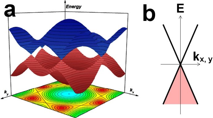
How can I create such a 3D plot using matplotlib? Like the one in Figure (a) below: 
I want to create it using DFT bandstructure calculation result
How can I create such a 3D plot using matplotlib? Like the one in Figure (a) below: 
I want to create it using DFT bandstructure calculation result
Consider a graphene Hamiltonian, whose dispersion looks a lot like the one in your figure. Per these notes, its k-space Hamiltonian may be written as: $$ H(k)=-t \sum_{\delta} [\cos(k\cdot\delta)\sigma_x-\sin(k\cdot\delta)\sigma_y], $$ where $k=(k_x,k_y)$, $\delta$ are nearest-neighbor vectors, $\sigma_i$ are Pauli matrices and $t$ is a hopping parameter. Please see referenced notes for vectors and other details pertaining to the model.
Per the time-independent Schrodinger equation, the energy dispersion you seek to plot comprises just the eigenvalues of the above Hamiltonian over some region of $k$-space. I will assume that you are working with an expression for the Hamiltonian (like the one above), instead of ab initio techniques. The given $2\times 2$ Hamiltonian is a $2$-level Hamiltonian that yields $2$ instantaneous eigenvectors/wavefunctions corresponding to $2$ eigenvalues. In your figure, the sets of eigenvalues pertaining to each eigenvector are given in two different colors (red and blue).
Therefore, you simply have to solve for the Hamiltonian's eigenvalues at each $k$-point in $k$-space. You may do this 'analytically' (to find expressions for the eigenvalues using algebra, that you can then plug $k$ points into), or 'numerically' (evaluating the Hamiltonian at each $k$ point first, to numerical get eigenvalues directly).
The 'analytic' method is just using some function $H(k)$ for the Hamiltonian to get an analytic expression for a different function $E(k)$ of the energy. You can plug $k$ into $E(k)$ to plot your figure. I personally prefer using Mathematica for this, because I like its in-build eigensystem-solving commands.
(* Define parameter space edges *)
BZx1=-1;BZx2=+1;BZy1=-1;BZy2=+1;
(* Define Hamiltonian *)
a = 2.46; t = 1; k = {kx, ky};
d1 = (a/2) {1, Sqrt[3]}; d2 = (a/2) {1, -Sqrt[3]}; d3 = -a {1,
   0};
sx = {{0, 1}, {1, 0}}; sy = {{0, -I}, {I, 0}}; (* Pauli matrices *)
hx = Cos[k.d1] + Cos[k.d2] + Cos[k.d3]; hy =
 Sin[k.d1] + Sin[k.d2] + Sin[k.d3];
H[kx_, ky_] = -t (hx*sx - hy*sy);
(* Get analytic expressions for energies *)
eigenvals[kx_, ky_] = Eigenvalues[H[kx, ky]];
(* Plot *)
Show[Plot3D[eigenvals[kx, ky][[1]], {kx, BZx1, BZx2}, {ky, BZy1, BZy2},
  PlotStyle -> Red],
 Plot3D[eigenvals[kx, ky][[2]], {kx, BZx1, BZx2}, {ky, BZy1, BZy2},
  PlotStyle -> Blue]]
This gives you:
I can imagine that a Sympy (+ matplotlib) approach would be similar. Additionally, I would not recommend trying to solve complicated expressions this way (unless you have the computational power).
On the other hand, the 'numerical' method requires first discretizing your $k$-space into a grid, and then plugging each grid point into $H(k)$ to get a matrix with numbers as its entries (as opposed to algebraic expressions). You can easily solve for the eigenvalues, and plot all resulting eigenvalue points to get a figure like the one you seek. Please bear in mind that eigenvectors are generally complex-valued, and that when using the numerical approach, different programs assign different arbitrary, complex-valued phases to each entry. This is not an issue in our case, as we care only about eigenvalues (which are real if dealing with a Hermitian system). I personally prefer using MATLAB or Python for this approach, because they are well-suited for working with numerical datasets.
The following code might look more complicated than it needs to be, but I like working with functions:
import numpy as np
from numpy import linalg as LA
import matplotlib.pyplot as plt

# First, define your Hamiltonian.
# The following function returns the Hamiltonian matrix for input (kx,ky).
def Hamiltonian_Graphene(kx,ky):
    a = 2.46 # Wikipedia
    t = 1
    k = np.array((kx,ky))
    d1 = (a/2)*np.array((1,np.sqrt(3)))
    d2 = (a/2)*np.array((1,-np.sqrt(3)))
    d3 = -a*np.array((1,0))
    sx = np.matrix([[0,1],[1,0]]);
    sy = np.matrix([[0,-1j],[1j,0]]);
    hx = np.cos(k@d1)+np.cos(k@d2)+np.cos(k@d3)
    hy = np.sin(k@d1)+np.sin(k@d2)+np.sin(k@d3)
    H = -t*(hx*sx - hy*sy)
    return H

# Onto plotting the dispersion.
# The parameters m,n specify the resolution to discretize the parameter space into (e.g. break it into m=10 pieces in the kx direction).
# The parameters BZx1,BZx2,BZy1,BZy2 specify the edges of your parameter space. I used BZx1=-1,BZx2=+1,BZy1=-1,BZy2=+1 in the
def plot_dispersion(m,n,BZx1,BZx2,BZy1,BZy2):
    # Generate a mesh
    kx_range = np.linspace(BZx1, BZx2, num=m)
    ky_range = np.linspace(BZy1, BZy2, num=n)
    # Get the number of levels with a dummy call (an NxN square matrix has N levels)
    num_levels = len(Hamiltonian_Graphene(1,1))
    energies = np.zeros((m,n,num_levels)); # initialize
    # Now iterate over discretized mesh, to consider each coordinate.
    for i in range(m):
        for j in range(n):
            H = Hamiltonian_Graphene(kx_range[i],ky_range[j]);
            evals, evecs = LA.eig(H); # Numerically get eigenvalues and eigenvectors
            energies[j,i,:]=evals;
    X, Y = np.meshgrid(kx_range, ky_range) # Generate actual mesh for plotting.
    # Plot! There are several ways to style this.
    fig = plt.figure()
    ax = fig.gca(projection='3d')
    ax.axis([X.min(), X.max(), Y.min(), Y.max()])
    transparency = 0.3 #transparency
    for band in range(num_levels):
        ax.scatter3D(X, Y, energies[:,:,band], alpha=transparency, antialiased=False, label="c")
    plt.show()

# Run it!
BZx1=-1;BZx2=+1;BZy1=-1;BZy2=+1;
plot_dispersion(100,100,BZx1,BZx2,BZy1,BZy2)
This gives you:
You might get an error ComplexWarning: Casting complex values to real discards the imaginary part, but that is because of rounding errors in Python (and can be avoided if you use np.eigh() instead of np.eig, if applicable). You can try to troubleshoot ways to get rid of this, and to make resulting figures prettier. I did not include the contour plot shown at the bottom of your figure, as it basically uses the same procedure.
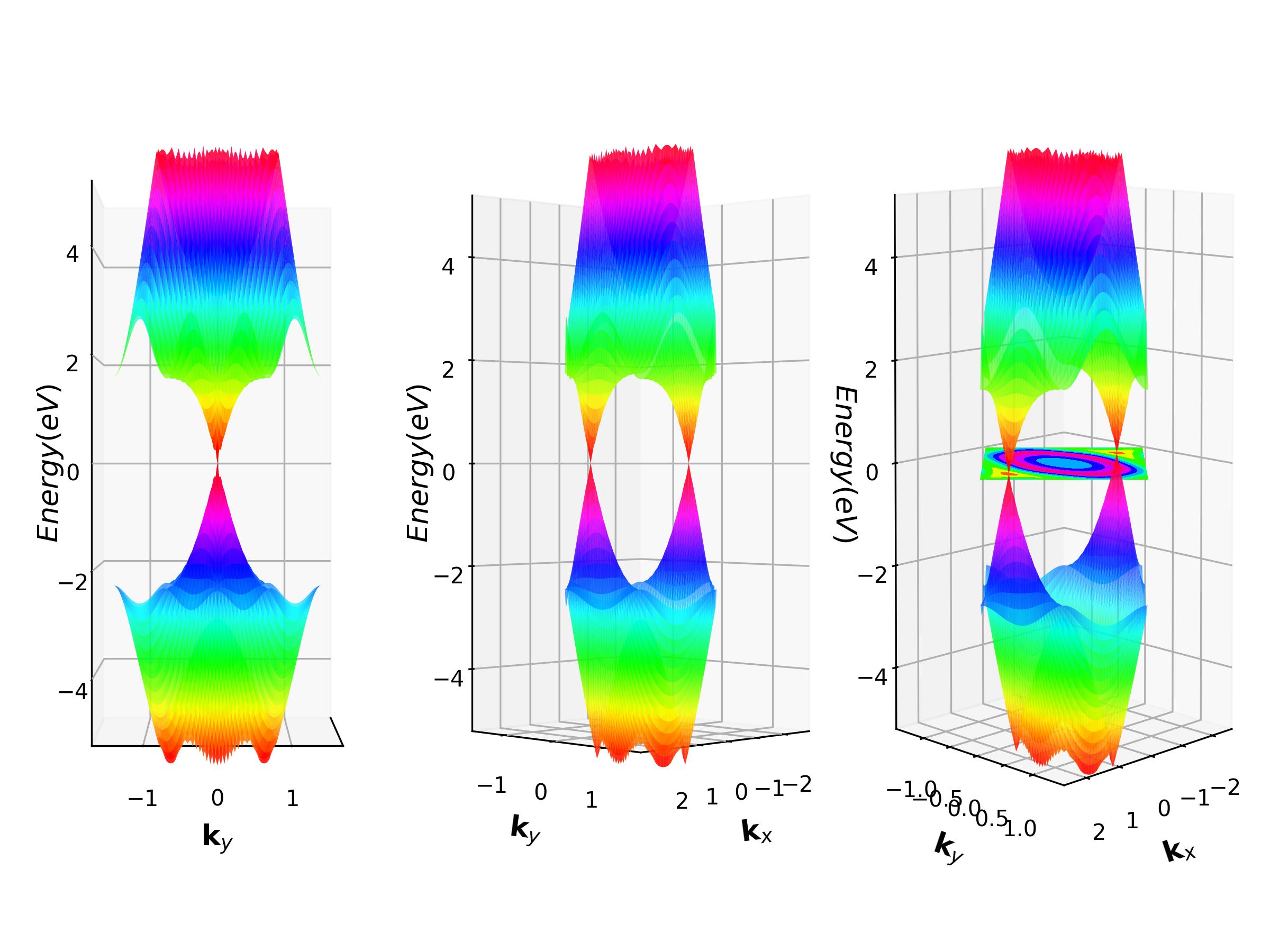
VASPKIT offers a tool to plot 3D band structure using VASP. The method select K-path on a surface of the Irreducilbe Brillouin zone and calculate the K-dependent band energies on those K-points. An example 3D plot of graphene bandstructure is shown below

For more details refer this tutorial
For a general case, create you input inside a loop:
Here, the mains steps are completely dependent on the DFT software you are using.