12
$\begingroup$

I am using an open source python package openmmtools to run a simple molecular simulation problem using the metropolis algorithm.

I first load a default system of particles (alanine-dipeptide in vacuum), add some uniform random disturbance to every position, then let the algorithm run to see if it brings me back to the starting system position.

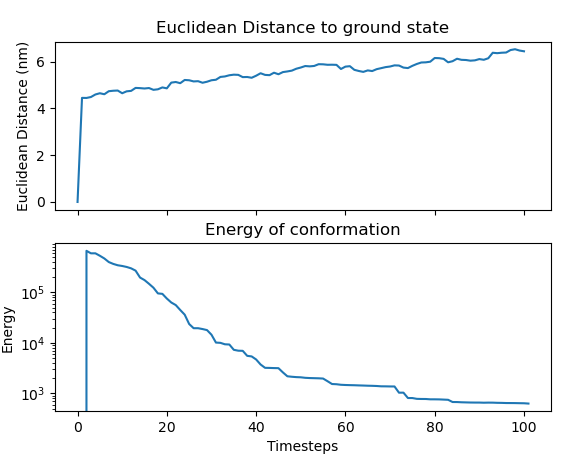
It looks like the metropolis moves decrease energy, as expected, but do not decrease the euclidean distance of each particle back to its starting position. Euclidean distance is just a sum of all the particle positions at any given state. The following graph is what I see when I measure these quantities. The big initial jump is when I add a disturbance to the positions of every particle in the system. I have even subtracted the mean of the particle positions from each particle to make sure that it isn't just that the entire system is shifting away from the starting position.

distance and energy during metropolis algorithm for simulation of 22 molecule system

Why do the Euclidean distances of each particle not decrease with the energy. In fact, they seem to increase as the simulation continues, which means the particles are growing farther and farther apart, which doesn't seem right. I know the molecule isn't rotating, since I'm drawing the state at each timestep as a 3D scatter plot and can see that it isn't.

I expect is something very silly on my end. I hope the confusion is clear.

Here's the code that gave me this graph, just in case.

from openmmtools import mcmc, testsystems, states, cache
from simtk import openmm
from simtk import unit
import numpy as np
import matplotlib.pyplot as plt


# user parameters
timesteps = 100
draw_init_final_positions = False
plot_distance_energy = True


class AddGaussianVector(mcmc.MetropolizedMove):
    def __init__(self, **kwargs):
        super(AddGaussianVector, self).__init__(**kwargs)

    def _propose_positions(self, initial_positions):
        # displacement = unit.Quantity(np.array([1, 1, 1]), initial_positions.unit)
        mean, var = 0, .1
        x_prop, y_prop, z_prop = np.random.normal(mean, var), np.random.normal(mean, var), np.random.normal(mean, var)
        displacement = unit.Quantity(np.array([x_prop, y_prop, z_prop]), initial_positions.unit)
        return initial_positions + displacement


def distance(x, correct):
    for k in range(3):
        x[:, k] -= np.mean(x[:, k])
        correct[:, k] -= np.mean(correct[:, k])
    noise = np.subtract(x, correct)
    return np.sqrt(np.sum(np.square(noise)))

platform = openmm.Platform.getPlatformByName('CUDA')
cache.global_context_cache.platform = platform

# Create the initial state (thermodynamic and microscopic) for an alanine dipeptide system in vacuum.
alanine = testsystems.AlanineDipeptideVacuum()
sampler_state = states.SamplerState(alanine.positions)
thermodynamic_state = states.ThermodynamicState(alanine.system, 300 * unit.kelvin)
e, d = [], []
context_cache = cache.global_context_cache
context, unused_integrator = context_cache.get_context(thermodynamic_state)
sampler_state.apply_to_context(context, ignore_velocities=True)
e.append(thermodynamic_state.reduced_potential(context))
d.append(distance(sampler_state.positions.copy(), sampler_state.positions.copy()))

# draw initial sampler_state
if draw_init_final_positions:
    plt.figure(1)
    ax = plt.axes(projection='3d')
    xdata = sampler_state.positions[:, 0]
    ydata = sampler_state.positions[:, 1]
    zdata = sampler_state.positions[:, 2]
    ax.scatter3D(xdata, ydata, zdata, cmap='Greens')
    plt.title('Initial particle conformation')


noise = np.zeros((sampler_state.n_particles, 3))
correct_state = sampler_state.positions.copy()
for i, molecule in enumerate(sampler_state.positions):

    # add noise to correct state
    noise_low, noise_high = -1, 1
    sampler_state.positions[i][0] += unit.quantity.Quantity(value= np.random.uniform(noise_low, noise_high), unit=unit.nanometer)
    sampler_state.positions[i][1] += unit.quantity.Quantity(value= np.random.uniform(noise_low, noise_high), unit=unit.nanometer)
    sampler_state.positions[i][2] += unit.quantity.Quantity(value= np.random.uniform(noise_low, noise_high), unit=unit.nanometer)

print('Correct_state: ', correct_state)
print('Noisey_state', sampler_state.positions.copy())
print('INITIAL DIST AND ENERGY: {} nm {} energy'.format(d[0], e[0]))

sampler_state.apply_to_context(context, ignore_velocities=True)
e.append(thermodynamic_state.reduced_potential(context))


# Create an update MCMC move that brings us back to the initial configuration.
current_state = sampler_state.positions.copy()
total_accepted, total_proposed = 0, 0

print('TOTAL PARTICLES: ', sampler_state.n_particles)
for ii in range(timesteps):
    for jj in range(sampler_state.n_particles):
        move = AddGaussianVector(atom_subset=[jj])
        move.apply(thermodynamic_state, sampler_state)
        if move.n_accepted == 1:
            total_accepted += 1
        total_proposed += 1

    current_state = sampler_state.positions.copy()
    # measure euclidean distance
    d.append(distance(current_state, correct_state))

    # measure energy
    sampler_state.apply_to_context(context, ignore_velocities=True)
    e.append(thermodynamic_state.reduced_potential(context))

fig, ((ax1),(ax2)) = plt.subplots(2, 1, sharex=True)
ax1.plot(d, label='Euclidean dist')
ax1.set_title('Euclidean Distance to ground state')
ax1.set_ylabel('Euclidean Distance (nm)')
ax2.plot(e, label='Energy')
ax2.set_yscale('log')
ax2.set_title('Energy of conformation')
ax2.set_xlabel('Timesteps')
ax2.set_ylabel('Energy')
ax2.text(2, 10, r'Original Energy {}'.format(e[0]), fontsize=15)
plt.show()

Edit: I've tried visualizing it as per a comment. I'm not sure if anything particular sticks out. The gif begins when the bottom left axis starts at -0.5.
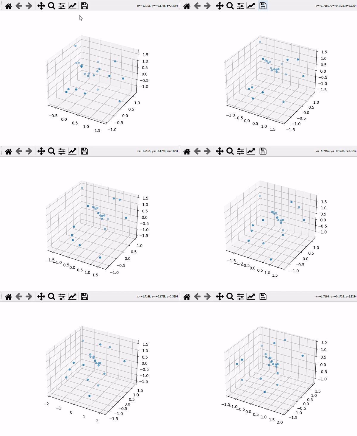
particles of alenine dipeptide as metropolis moves are applied

$\endgroup$
5
  • 1
    $\begingroup$ I think the easiest way to see what's happening is to output a trajectory and visualise it in e.g. PyMOL. Sometimes there could be an error in the analysis, rather than the simulation and visualisation makes the analysis a bit easier and less prone to errors. $\endgroup$
    – Godzilla
    Commented Mar 8, 2021 at 0:27
  • 3
    $\begingroup$ Also, in this setting MCMC is a sampling, rather than optimization algorithm so you can't expect the MCMC structures to match your initial one. On the contrary, I'd expect the conformation to diverge over time and sample states of high conformational entropy instead $\endgroup$
    – Godzilla
    Commented Mar 8, 2021 at 0:32
  • $\begingroup$ The distance will probably also converge before too long. There is effectively a temperature in MCMC, so the system will fluctuate around some average geometry. Depending on what states are accessible, this average geometry may be fairly close to the initial geometry, but the energy and distance will never instantaneously return to the initial values. $\endgroup$
    – jheindel
    Commented Mar 8, 2021 at 23:24
  • $\begingroup$ I see. Since temperature may be setting the average geometry, I lowered the simulation temperature to 1 kelvin. It still doesn't seem to change the results in any significant manner i.e distance still increases and energy decreases very similarly to above. Godzilla, if it were sampling high conformational entropy states, would it not show in the energy plot above? I'll try running the simulation for longer and come back with an update! $\endgroup$
    – Squishy
    Commented Mar 9, 2021 at 15:59
  • $\begingroup$ Please do not cross-post to/from other sites of the network. I will delete the corresponding post on Chemistry. $\endgroup$ Commented Jan 12, 2022 at 19:42

1 Answer 1

9
$\begingroup$

Most of the problem here appears to be because constraints in the test system default to app.HBonds, which means all bonds to hydrogen atoms are constrained. Something goes very weird when you force a large, unphysical change on the system, and then try to apply HBond constraints (it looks to me like it isn't even constraining HBonds to the unphysical lengths; there's probably a limitation in the constraint algorithm).

On the other hand, by creating the test system with:

alanine = testsystems.AlanineDipeptideVacuum(constraints=None)

I got following at frames 0, 25, and 100:

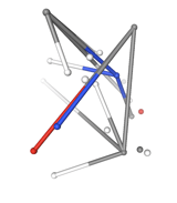
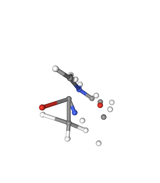
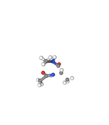
Frame 0Frame 25Frame 100

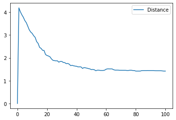
That's starting to look a decent bit like alanine dipeptide. Here's the 'distance' plot:

distance

By the way, you may be making another assumption that isn't quite true: don't assume that the distance will go to zero. You've done nothing to align your atoms with the reference structure. I think what you're really wanting to look at is a root-mean-square-deviation (RMSD) calculation, which would include that alignment. Tools like MDTraj and MDAnalysis implement RMSD and related algorithms.

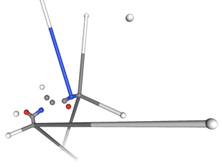
As suggested in the comments, it's easier to see what was going wrong if you use a tool that is designed for visualizing chemical structures, instead of just a 3D scatterplot. Much of the backbone is in place even with constraints. Godzilla mentions PyMOL in the comment. I used NGLView. Here's what I saw with constraints after 100 steps:

with_constraints

The bonds to hydrogens are clearly all wrong, but the heavy atoms look pretty much like alanine dipeptide. Having the atom colors (and, in my notebook, the atom labels when I hover over them) makes it much easier to diagnose the issue.


Addendum: To get from a list of positions to a visualization in NGLView, the process I used is: data $\to$ MDTraj $\to$ NGLView. The data you need is a list of snapshot coordinates, so I modified the OP code to save current_state at every frame in a list called trajectory (same as how energies are saved in e and distances saved in d). From there it is really easy, because OpenMMTools test systems are designed to integrate with MDTraj (and so is NGLView):

import mdtraj as md
import nglview as nv

# alanine is the openmmtools testsystem
# trajectory is a list or np.array with shape (n_frames, n_atoms, 3)
# no explicit units; values in nm
traj = md.Trajectory(trajectory, topology=alanine.mdtraj_topology)
view = nv.show_mdtraj(traj)
view  # return the view so it is shown in notebook
# get the image for a specific frame number
view.frame=25
view.download_image("frame25.gif")

A few points on that:

  1. Installing NGLView for classic Jupyter notebook often requires the command jupyter-nbextension enable nglview --py --sys-prefix after a conda/pip install to enable it. Installing NGLView in Jupyter Lab is a little messier (see this script; currently [March 2021] NGLView does not yet work with Jupyter Lab 3.0).
  2. The topology is how MDTraj knows what each atom is and what bonds there are. I think that some bonds are not shown because either MDTraj or NGLView refuses to believe that they could actually be bonds, based on the initial configuration. If you weren't using OpenMMTools, you could get an MDTraj topology from an OpenMM topology with md.Topology.from_openmm, or you could save to a file that contains topology information and load that in MDTraj with md.load(filename).
  3. You could use other visualization tools (PyMOL, VMD, etc) by using traj.save('filename.pdb') and loading the PDB trajectory in the other tool. (I suggest PDB here because it includes topology information and is widely supported; many other formats are more efficient on disk but require a separate file for topology.)
$\endgroup$
5
  • $\begingroup$ +1 Amazing! This question came from Chemistry.SE and I wasn't sure if we had enough people to give a good answer to the user in a timely manner since Chem.SE has so many more users than us. Thanks so much for your contributions here! $\endgroup$ Commented Mar 9, 2021 at 19:15
  • 4
    $\begingroup$ @NikeDattani Glad to help! I used to work in the group that develops OpenMMTools and I have contributed a few lines of code to it, so when I saw a question on it, I thought I'd see if I could find an answer. $\endgroup$
    – dwhswenson
    Commented Mar 9, 2021 at 19:25
  • $\begingroup$ Thank you! This does make sense. Would you by chance know of any resources where I could learn to use nglview to visualize the sampler_states in openmmtools? If it's possible to share your code to do this it would be hugely helpful. Thanks for spending the time to answer my question! $\endgroup$
    – Squishy
    Commented Mar 11, 2021 at 4:29
  • 1
    $\begingroup$ @Squishy: Updated with an addendum on how to do that (it's really easy when using OpenMMTools test systems -- the hardest part will be getting NGLView installed) $\endgroup$
    – dwhswenson
    Commented Mar 11, 2021 at 10:53
  • $\begingroup$ @Squishy I think that follow-up question should be asked as a separate question in a separate post, rather than in a comment. $\endgroup$ Commented Mar 11, 2021 at 15:41

You must log in to answer this question.

Not the answer you're looking for? Browse other questions tagged .