How to choose half-Brillouin-zone (HBZ) in Fukui & Hatsugai's numerical scheme for the Z2 invariant?

Question

EDIT: Please see my first comment on this question first.

---

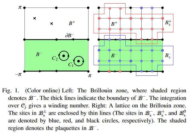
In this paper, Fukui and Hatsugai present a numerical scheme for the calculation of the $\mathbb{Z}_2$ index that uses the following definition: $$\tag{1} \mathbb{Z}_2 = \frac{1}{2\pi}\left[ \oint_{\partial HBZ} A dk - \int_{HBZ} \Omega_z d^2k \right] (\text{mod } 2). $$ In Figure 1 of the paper (screenshot below), they identify three types of $k$-points in a discretized Brillouin zone lattice. These three sets are denoted by $\mathcal{B}_s^\pm$ and $\mathcal{B}_s^0$. They define what each of these points are:

• $\mathcal{B}_s^0$ are time-reversal $\mathcal{T}$-invariant sites: $\mathcal{T}H(k_l)\mathcal{T}^{-1}=H(k_l)$.
• As a $\mathcal{T}$ constraint, states at $-k_l\in\mathcal{B}_s^+$ are Kramers doublets of states at $k_l \in \mathcal{B}_s^-$.
• If the spectrum at each $k_l$ is arranged as $\epsilon_n (k_l)\leq\epsilon_{n+1}(k_l)$, the states at $-k_l$ can be constrained as: $|n(-k_l)\rangle=\mathcal{T}|n(k_l)\rangle,$ for $k_l\in\mathcal{B}_s^-$.
• Both Kramers doublets are included in $\mathcal{B}_s^0$. Arranging the spectrum here as $\epsilon_{2n-1}(k)= \epsilon_{2n}(k)\leq \epsilon_{2n+1}(k)$, they impose a final constraint: $|2n(k_l)\rangle=\mathcal{T}|n(k_l)\rangle$, for $k_l\in\mathcal{B}_s^-$.

They use these constrained states to define a link variable per the usual Fukui-Hatsugai-Susuki scheme (I think). I have implemented this common scheme in Python and MATLAB with no issue, but I am having trouble imposing the required constraints and properly choosing one half-Brillouin-zone for eq. $(1)$ above. I can see it being easy to do with some hard-coding in a low-resolution lattice, but I was wondering whether someone give me insight on translating the above constraints to code, and properly choosing the three different types of $k$-points ($\mathcal{B}_s^i$) automatically without hard-coding. Thanks.

Answer 1

I think I figured this out. For most practical purposes, I think it is fine to just choose $-\pi\leq k_x\leq \pi$ and $0\leq k_y\leq \pi$ (half-BZ, with exact ranges depending on the model). I think I over-complicated the authors' work. It is unlikely that the vortices/singularities will occur near the boundary of the chosen region. So, I can just take the difference between the Berry connection and curvature integrals. If the singularities do occur near the boundary, I think it is okay to offset the region of integration in a consistent manner to avoid having to choose the region of integration so carefully as in Figure 1. Someone please correct me if I am wrong. Thanks.